Introduction
The task at hand is simply to evaluate an integral of the type:

where the one-dimensional function  and the integration
limits are selected by the user. In general the limits
and the integration
limits are selected by the user. In general the limits  and
and
 may be at infinity and the function may have
singularities. These possibilities substantially complicate the
algorithms for evaluating the integral.
may be at infinity and the function may have
singularities. These possibilities substantially complicate the
algorithms for evaluating the integral.
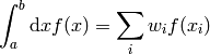
The result of the integral is typically evaluated simply as a weighted
linear sum of values of the function at a number of
points  :
:
The main logic in these algorithms is then to:
- Decide at which points to evaluate the function
- Decide the optimal weighing factors for the problem at hand
It is clear that short of making the set of  the entire
available space of machine numbers, a specially crafted (probably
non-smooth) function could make any particular algorithm produce a
badly incorrect answer. In other words, for a completely general
function, no guarantee can be made about the accuracy of any
algorithm.
the entire
available space of machine numbers, a specially crafted (probably
non-smooth) function could make any particular algorithm produce a
badly incorrect answer. In other words, for a completely general
function, no guarantee can be made about the accuracy of any
algorithm.
For this reason, one-dimensional integration algorithms are usually classified by specifying the family or families of functions for which they in fact give the exact answer (obviously to within the limits of numerical precision).
Links: