An update on visualising the computational graph of a jax program
I’ve written while ago about visualising the computational graph of a JAX program here. Jax has evolved since then, so here is an update for the current (as of time of writing) version of Jax (0.3.1).
Export the HLO Intermediate Representation (IR)
The main change is that the graph is produced from an
jax.xla_computation object. The other change is that instead of
specifying the input shape I am supplying an example array
(numpy.ones(100)).
Here is the updated program:
import jax
from jax import numpy, grad

def tanh(x):
  y = numpy.exp(-2.0 * x)
  return (1.0 - y) / (1.0 + y)

def lfn(x):
    return numpy.log(tanh(x).sum())

def dlfn(x):
    return  grad(lfn)(x)

z=jax.xla_computation(dlfn)(numpy.ones(100))

with open("t.txt", "w") as f:
    f.write(z.as_hlo_text())
This will create a text file t.txt with a text-based HLO.
Visualise
The simplest way of visualising is to dump as a dot graph and run dot:
with open("t.dot", "w") as f:
    f.write(z.as_hlo_dot_graph())
dot t.dot -Tpng > t.png
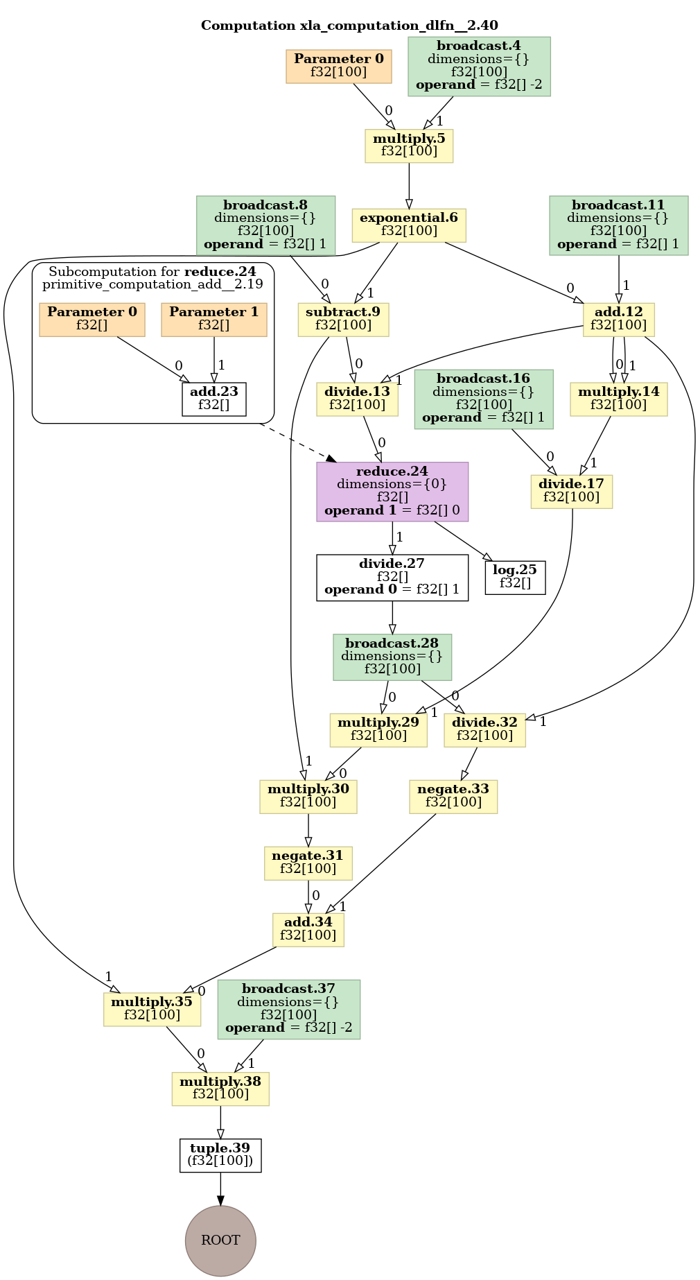
This produces the following image:
Visualise the optimised graph
(added on 2023-08-28 )
It is possible to also visualise the optimised graph produced by the XLA compiler.
The mechanism to get the HLO representation of a compiled graph is
shown in test_compiler_ir test in file api_test.py of the JaX
repository. Basically it consists of calling the jax.jit
function, lower()ing using to a specific example data structure
as argument, compile()ing and then using the as_text()
method. So for example:
def ff(x):
    x = x*3
    x = x+2
    return x

jax.jit(ff).lower(numpy.ones(100)).compile().as_text()
To visualise it is necessary to re-parse the HLO into a XLA computation and then use the XLA functionality to generate a Dot graph. This can be easily achieved using the raw XLA Python bindings with following function:
def todotgraph(x):
   return xla_client._xla.hlo_module_to_dot_graph(xla_client._xla.hlo_module_from_text(x))
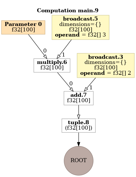
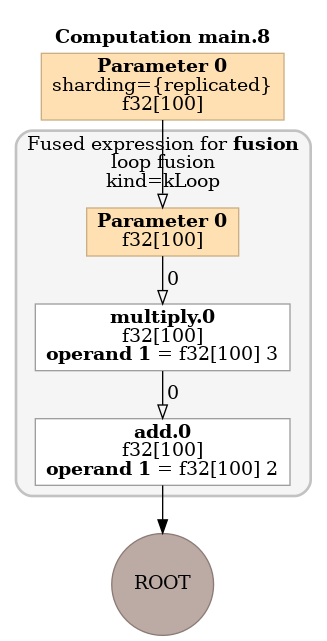
As an example for the above function the compiled graph shows XLA loop fusion. The un-optimised graph needs two loops over arrays:
But the optimised graph using the jit compiled function only needs one:
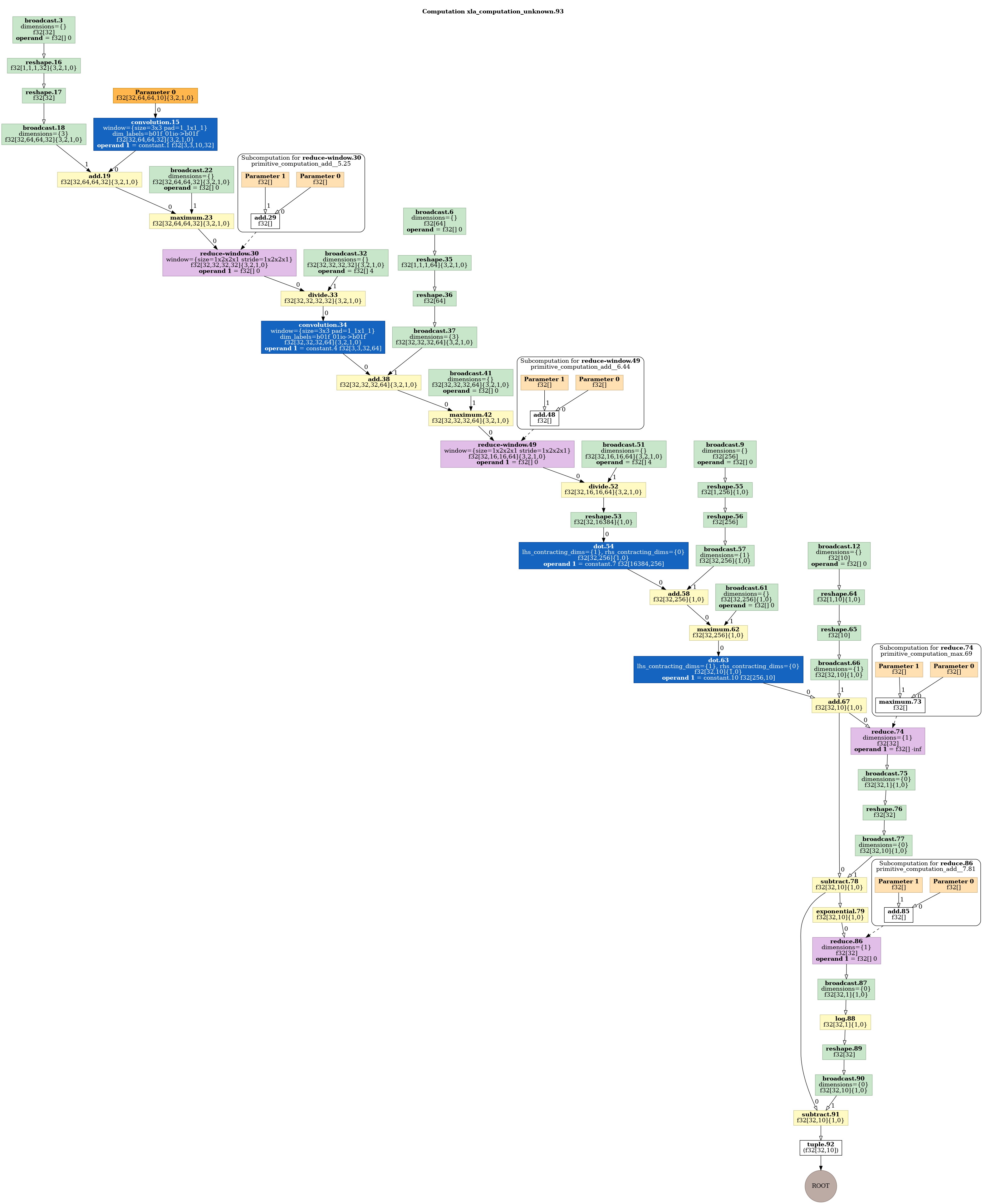
Visualise a neural network
The same basic approach can be used to visualise a flax neural network, e.g.,:
import functools
import flax.linen as nn

class CNN(nn.Module):
  @nn.compact
  def __call__(self, x):
    x = nn.Conv(features=32, kernel_size=(3, 3))(x)
    x = nn.relu(x)
    x = nn.avg_pool(x, window_shape=(2, 2), strides=(2, 2))
    x = nn.Conv(features=64, kernel_size=(3, 3))(x)
    x = nn.relu(x)
    x = nn.avg_pool(x, window_shape=(2, 2), strides=(2, 2))
    x = x.reshape((x.shape[0], -1))  # flatten
    x = nn.Dense(features=256)(x)
    x = nn.relu(x)
    x = nn.Dense(features=10)(x)
    x = nn.log_softmax(x)
    return x

model = CNN()
batch = numpy.ones((32, 64, 64, 10))  # (N, H, W, C) format
variables = model.init(jax.random.PRNGKey(0), batch)

f=functools.partial(model.apply, variables)
z=jax.xla_computation(f)(batch)

with open("t2.dot", "w") as f:
    f.write(z.as_hlo_dot_graph())
This produces the following image: